• 4-minute read
• 26th July 2021

A Quick Guide to Formatting Text in Microsoft Excel

Changing the appearance of the text in a spreadsheet can make it easier to read. But how do you adjust the font, size and colour of the text? And how do you apply effects? In this article, we provide a quick guide to formatting text in Microsoft Excel.

How to Adjust Fonts in Excel

To change the font used in a cell in Microsoft Excel, you will need to:

1. Select all of the cells that you wish to format with the cursor.
2. Go to the Home tab on the main ribbon.
3. Click the fonts dropdown (i.e. the menu with the name of the current font in it).
4. Select the font you want to use from the list.

This will automatically change the typeface for any text already in the selected cell(s), plus any text later typed into the formatted cell(s).

Changing the Font Size in Excel

To change the font size in Microsoft Excel, all you need to do is:

• Select the cell(s) you want to format with the cursor.
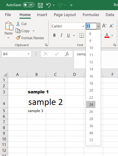
• Click the font size dropdown on the Home tab of the ribbon (i.e. the dropdown next to the main font menu).
• Select a value from the list to adjust the size of the text in the selected cell(s).

You can also increase or decrease the font size by one step via the capital ‘A’ buttons with up and down arrows next to this dropdown.

Changing the Font Colour in Excel

To change the font colour in Microsoft Excel:

• Select the cell(s) you want to format.
• Click the font colour button on the Home tab (see below).
• Select a colour from the options available (or click More Colors… at the bottom of this menu to open a new pop-up with custom colours).

You can also change the background colour of a cell by using the Fill Color option to the left of the font colour menu (i.e. the paint bucket icon).

How to Apply Effects in Excel

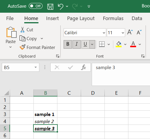
In Excel, you can also apply italics, bold, and underlining to text. These effects can all be found next to each other in the font group of the Home tab.

To apply your preferred style(s), select the cell(s) you wish to change, and then click on the B for bold, I for italics or U for underlining. 

You also add strikethrough, subscript or superscript to text in Excel.

To do this, click the arrow in the bottom right of the font group to open the Format Cells pop-up. Make sure the Font tab is selected, then select your required formatting from the options in the Effects section of the window.

You can make changes to the font, font size, and font colour from this pop-up window too, if required, though it is usually quicker to do it via the Home tab.

Formatting Part of a Cell

Finally, what if you want to format a specific part of the text within a cell rather than all the text in a cell? Here’s how you do this:

1. Select the cell with the text you want to format.
2. In the formula bar, select the specific text you would like to change.
3. Choose your preferred formatting using the options set out above.

The change will then be applied in the selected cell, but not in the formula bar.

Expert Spreadsheet Proofreading

Hopefully, this post has explained some of the basics of formatting text in Excel. But you’ll also want the text in your spreadsheets to be error-free. Why not send in a document today and have it checked by our spreadsheet experts?